-
Part 3 – One Stream At A Time
The third part of the story of the restoration of the turquoise darter in Sixmile Creek was initiated after the darters had become established and were abundant. There was very little previously published about the life history of the turquoise darter in the decades since its initial description as a species. Reasons for this are related to the fact that it is a small non-game species with no sport or economic value and that it is limited to the Savanah River drainage of South Carolina and Georgia. Darters of course have ecological value. They are indicators of stream health. They are sensitive to change in water quality. That is why they are typically the first species to disappear from a polluted creek, stream or river.
The third graduate student was Steph Irwin.

Steph Irwin recording data during darter field sampling in the Clemson Forest. His thesis would determine the timing of the turquoise darter’s spawning, the fecundity (number of eggs produced) of females, and the abundance of the darters on Sixmile Creek’s riffles measured in number of fish per unit area. This would require sampling the darters periodically over the course of a year and utilizing “depletion” sampling to ascertain abundance.
Depletion studies sounds ‘bad” but in fact all it involves is thorough sampling of a section closed with upstream and downstream block nets and briefly holding the fish captured on each pass in tanks representing the first, second, third and perhaps fourth pass.

Above: Clemson Undergraduates providing needed “manpower” to completely sample Sixmile Creek bank-to-bank. Below: The nets are placed downstream of the positive wand of the DC current electrofished and the darters drift from their hidden places in riffle into the nets. 
Darters captured in each successive pass of “depletion study” are held separately and enumerated before being returned to their riffle. The fish are enumerated. The theory is that as you capture most of the fish with each successive pass the catch per unit effort (CPUE) goes down with each pass. If this happens a depletion abundance estimate can be made by extrapolation to zero CPUE.

Example from actual data that shows how a depletion study does not need to sample all the fish in a closed section, but can predict how many fish are there based upon a negative slope and projection of K to zero CPUE
The fish are returned unharmed to the stream less than an hour after capture. In order to sample the entire stream with each pass students in my wildlife fisheries classes provided the “manpower” needed to cover the stream left to right.
In order to determine timing of spawning and fecundity a periodic small sample of darters had to be captured and sacrificed in order to measure the size of their gonads and egg counts.

Winter sampling for reproductive cycle timing data. All work was performed with approved Clemson University Institutional Animal Care and Use Protocols.
Darter density on Sixmile Creek’s riffles was 0.37 per meter squared. This is equal to 3691 per hectare and compares to Jay Delong’s estimate of 2799/ha for Twelve Mile Creek. This compares to reports for other darter species in other states where values ranged from 0.17 to 0.42 darters per square meter.

A male turquoise darter in Sixmile Creek. 
GSI is the gonadosomatic index of darters from January to June.
GSI peaked in mid to late April (above). The percentage of ova that were mature also peaked in late April to mid May (below). Clearly, the darters spawn in late April and early May.

Jay Delong’s M.S. thesis research provided data to predict the habitat needed by turquoise darters. Kevin Kubach’s M.S. thesis used Jay’s data to develop and implement a model for restoration of darters to Sixmile Creek in the Clemson Forest. Steph Irwin’s M.S. thesis evaluated the status of the darters following restoration efforts and described the reproductive cycle of the darter. Fellow faculty and working professionals who had graduated from Clemson Wildlife helped out on darter restoration sampling. More than 200 Clemson Wildlife and Environmental Science undergraduates assisted in field sampling Sixmile Creek and its darters over a period of more than ten years. Jay Delong (deceased) would be pleased that his work was used. Kevin and Steph are working professionals. I am retired. The darters are abundant.
-
PART 2 – One Stream At A Time – The Restoration of Darters To Sixmile Creek
Kevin Kubach was the second graduate student whose M.S. Thesis was part of the Turquoise Darter Restoration in Sixmile Creek. Kevin’s thesis involved surveying the physical and chemical habitat of Sixmile Creek in the Clemson Forest and computing the habitat suitability using Jay Delong’s graphs. Hundreds of transect were established at regular intervals and the stream’s characteristics (e.g., depth, water velocity, substrate) were measured at one-meter intervals across the transects. The stream was mapped dividing it into riffles (darter’s preferred habitat), runs (deeper and slower than riffles) and pools.
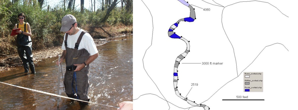
Kevin measuring stream habitat along a transect. After determining that Sixmile Creek would provide suitable habitat for the turquoise darter the next phase of Kevin’s thesis was designing a “re-introduction” plan. The plan chosen was to capture turquoise darters from tributary of nearby Twelve Mile River during the month of February and transport them to Sixmile Creek. February was chosen as the month because the water temperatures were at the coolest point of the year and dissolved oxygen was highest. We knew the darters spawned sometime later in the spring so the female’s ovaries and the male’s testes should not be fully “seasonally-developed.” If they were fully developed there would be the risk of the fish releasing their eggs and milt prematurely due to capture and handling. The initial plan was to transfer about 100 darters each February for about 10 years. Each transfer would be made to a riffle area further upstream from the previous year’s riffle. The stream selected as the source of darters had a history of high abundance of turquoise darters. We would monitor catch per unit effort (CPUE) at the source stream (Prater’s Creek) each year. CPUE did not decline over the stocking years so we were not concerned that we were depleting the darters in Prater’s Creek. The source site was located in the middle of Prater’s Creek. We moved 637 darters between 2003 and 2010. The 2009 and 2010 stockings were lower in number. Field trips with Clemson classes after 2005 showed that the darters were well-established. Generally we captured roughly 50 darters below the Belle Shoals Road bridge (34.84 N lat, -82.75 W lon) and then a day or two later 50 from upstream of the bridge. Beginning in 2006 we released darters further upstream in Sixmile Creek at Old Seneca Highway because antidotal reports in the literature suggested young-of-the-year darters drift downstream. Finally, Kevin and I would sample Sixmile Creek downstream of the re-introduction riffles in July of the first summer when young-of-the-year (Y-O-Y) darters should be about 1 cm in length. In fact we did capture some Y-O-Y darters that first summer. We were excited because we knew the darters place in Sixmile Creek five months prior had spawned. That first Y-O-Y darter we captured was so small that at first glance we thought we had a Mayfly (insect) nymph in the net.
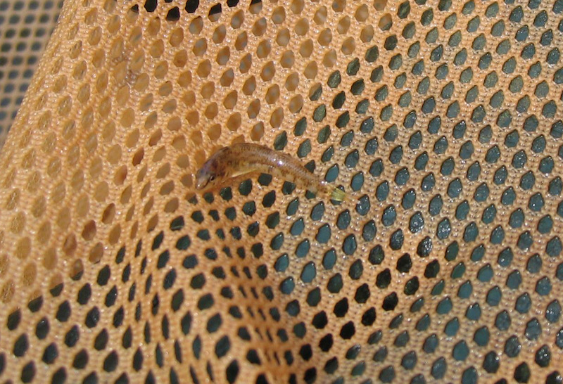
A Young-Of-The-Year Darter (first time in perhaps 70 years) My fisheries classes would then sample monthly August through April each year and records of darter captures were recorded. Any darters captured were released since they would represent the “newly-established”, re-introduced darters. Annual February transfers of darters took place for six years. Kevin who was now working for SCDNR and I conducted the annual transfers. Former and current students, faculty and staff, and would assist with the annual transfers in February. Annual transfers were stopped when darter captures during Clemson class field trips on Sixmile Creek indicated that turquoise darters had achieved substantial abundance. They became very abundant on the riffles and the third student’s MS Thesis would determine what their density was per unit area of riffle, and the timing of their reproductive cycle (next week).
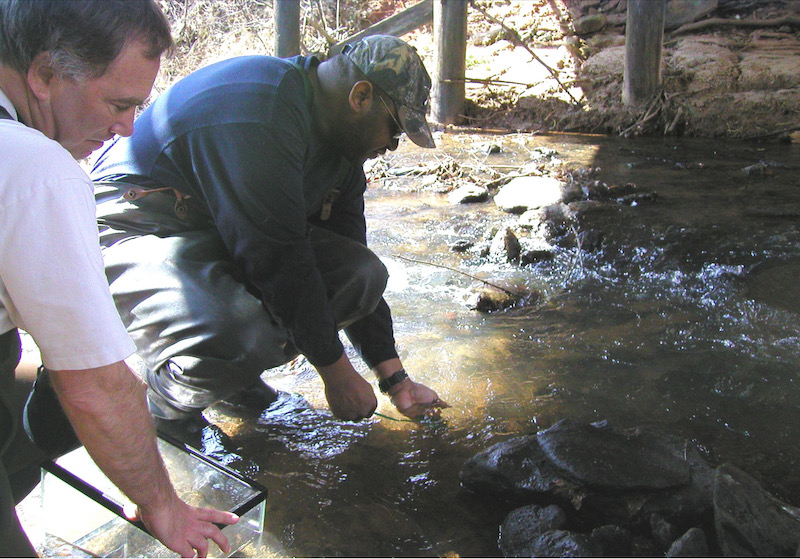
Professor Drew Lanham assists with a darter stocking. -
One Stream At A Time
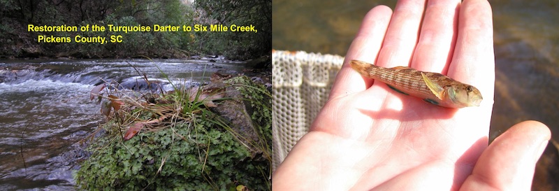
Sixmile Creek And The Restored Turquoise Darter In the 100 years after the civil war we lost countless small streams and rivers to agriculture and urbanization one stream at a time over 1000’s and 1000’s of landscapes in America. This is the story of restoration of one of those streams, Sixmile Creek. Earth Day 2022 was Friday April 22 so this and the next blog will cover efforts by me and my graduate students to make earth a little better, one stream at a time.
By the time the Great Depression (1929-1939) happened much of the agricultural lands in the southeast U.S. and Midwest U.S. were in just as bad condition as the U.S. economy. Agricultural practices in the late 1800’s and early 1900’s had depleted soils of the characteristic which sustain agriculture. After the Civil War nearly 2/3rds of farmlands in the upstate of South Carolina were farmed by tenant farmers and sharecroppers who did not own the land and had no incentive to protect the land for future generations. The percentage of lands converted from forests to agriculture peaked. Across the South and the Midwest, a terrible drought struck. The years 1930 and 1931 had been unusually dry, but 1934 brought drought to 80 percent of the U.S., and extreme drought returned in 1936, 1939, and 1940. Soil erosion was widespread. There were no systematic studies made during those years so scientists can only speculate about stream and river water quality.
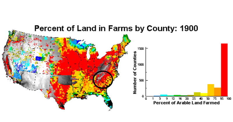
By 1900, most lands in upstate South Carolina were being farmed. President Roosevelt signed the Bankhead-Jones Farm Tenant Act in 1937. The purpose of the law included the ability of the federal government to purchase “sub-marginal” lands no longer fit for agricultural use and then utilize that land for other more suitable purposes including conservation programs.
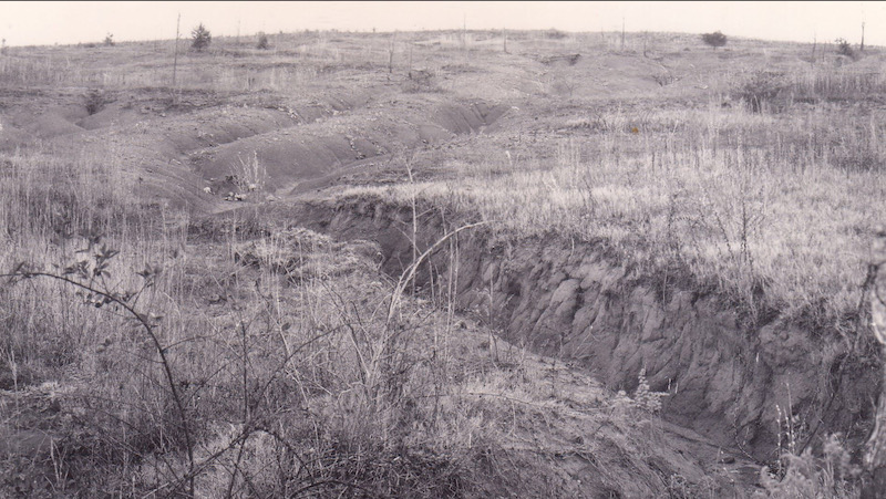
Photograph from 1930 of marginal farmland near what is now the Clemson Experimental Forest. The history of the Clemson Forest was rooted in the Great Depression of the 1930’s. It was the efforts from Dr. George Aull (Agricultural Economics) that got the whole thing started. The Clemson Experimental Forest is the product of the “Clemson Community Conservation Project” (CCCP) initiated by Dr. Aull.
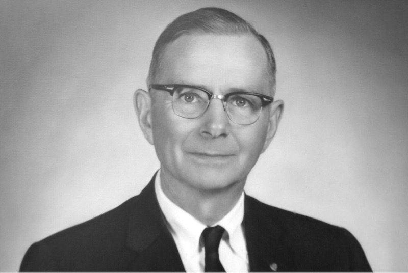
Dr. George Aull The Project was funded by the Roosevelt Administration’s New Deal programs, and later by the Bankhead – Jones Farm Tenant Act. Nearly 30,000 acres of worn out farmlands around Clemson College were purchased under the project. Then, in 1954, the project was deeded to Clemson College, thanks to the efforts of U.S. Senators Charlie Daniel, Strom Thurmond, State Senator Edgar Brown and Dr. George H. Aull. The Clemson Experimental Forest was born.
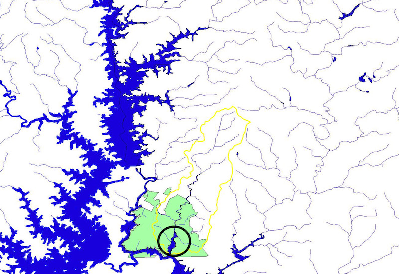
The “north forest” of Clemson University’s Experimental Forest (green), Sixmile Creek’s drainage basin (yellow outline) and Issaqueena Lake in circle. Upper Lake Hartwell (formerly Keowee River) to the left of forest and Lake Keowee on left side of map. All across the Southeast U.S. damaged lands also damaged small streams which lost their riparian vegetation. The riparian vegetation stabilized stream side soils and kept streams cool because of shade provided by the trees. The vegetation was also the fuel for the stream food web. Food webs in stream ecosystems were not understood until the 1970’s. After the abandonment of farms many lands underwent secondary succession and slowly recovered; and so did the water quality of their streams. The CCCP included reforestation efforts of the lands around Sixmile Creek. Small tributaries in areas which were too steeply-sloped for farming provided safe haven for some but not all fish species to re-populate recovering streams. Downstream rivers also provided a means for tributary streams to recover fish species providing no impediments for upstream migration were constructed.
Sixmile Creek was a special situation as were so many other streams in the U.S. During the Great Depression and decades before reforestation had a chance to improve stream water quality and habitat a reservoir was built near the confluence of Sixmile Creek with the Keowee River. The dam was a Civilian Conservation Corps (CCC) (1933-1942) project to put unemployed persons to work. The dam created Lake Issaquena (1934). But the dam also prevented migration of fish from the Keowee River back into Sixmile Creek. The timing could not have been worse. At the precise time when the landscape would begin a multi-decade healing process the dam was created where the stream entered the Keowee River. The dam permanently isolated Sixmile Creek from all other riverine ecosystems. In nature and undisturbed by man, riverine ecosystems are a complex network of inter-connected, flowing waters which transport water and materials downstream collecting into larger streams and rivers. But passage by fishes is possible in both directions. Then in the mid-1950’s Lake Hartwell’s dam impounded the Seneca River, the lower Keowee River and lower Twelve Mile River. But the Issaqueena Dam was impassable for fish, so Lake Hartwell did not directly impact Sixmile Creek because it was preceded by the Issaqueena Dam. The lands surrounding Sixmile Creek had experienced agricultural abuse in the 1800’s and early 1900’s and some fish species losses were now permanent because of Sixmile Creeks isolation created by the presence of Lake Issaquenna and its dam.
When I started teaching at Clemson University in 1978 only one other fisheries Professor had preceded me in that position. He had made several fish collections in Sixmile Creek and surrounding streams. His specimens were deposited in the Fish Collections of the “Vertebrate Museum” at Clemson University. The SC DNR biologist with an office near Clemson had a primary responsibility as “Trout Biologist” which meant his efforts focused on the trout waters in SC’s mountains. I was teaching Ichthyology in one semester and Fishery Biology during the other semester. Both classes included weekly field trips. So I set about sampling the streams of Pickens County including Sixmile Creek in Clemson’s Experimental Forest. After about 20 years of sampling I thought it was peculiar that Sixmile Creek was missing the the two species of darters found in all surrounding streams and rivers: turquoise darters and blackbanded darters, particularly the turquoise darter which thrived in similarly sized streams nearby. Later when I considered the history of Sixmile Creek it all made sense. In 1990 my first student working on darters (Jay Delong, M.S. 1991) developed “Habitat Suitability” models for the Turquoise Darter and several other small non-game species using a pristine tributary of Twelvemile River.
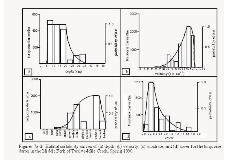
Jay Delong’s MS Thesis developed “Habitat Suitability Curves” for several species of small non-game fishes including the Turquoise Darter. Habitat Suitability models show preferred habitat characteristics of a species. The models are built by tedious sampling of small quadrants or plots of a stream and comparing the abundance of the species in question to the habitat characteristics for that plot. The primary habitat characteristics measured are substrate, depth, and velocity providing temperature and oxygen are suitable. “Habitat Suitability” models were being developed all across the country for the purpose of regulating or maintaining minimum discharges below hydroelectric dams in order to provide habitat for fish species. Jay’s Delong’s Habitat Suitability models would be used by my second student to evaluate Sixmile Creek’s habitat suitability for restoration of Turquoise Darters, design a “re-introduction plan” and initiate the plan (next blog).
-
The Easter Bunny Should Have Been “The Easter Echidna”
Easter Bunnies being typical mammals don’t lay eggs despite the traditions of German immigrants. In the 1700s German immigrants to Pennsylvania (who also brought us the tradition of “Groundhog Day”) brought over their tradition of an egg-laying hare named “Osterhase” (pronounced “Oschter Haws”). Legend has it, the rabbit would lay colorful eggs as gifts to children who were good, so kids would make nests in which the bunny could leave its eggs. The custom spread across America and became a widespread Easter tradition. Over time, the Easter bunny’s delivery expanded from just eggs to include other candy treats such as chocolate and toys.
An Echidna, an egg-laying Mammal. Like most mammals, bunny rabbits are viviparous (from latin, vivi = live; and parire “to bring forth” or birth). There are a few egg-laying mammals, but they are in Australia and New Guinea. In fact, only five living species of mammals are not live-bearers: the egg-laying duck-billed platypus and four species of echidna (also known as spiny anteaters). Egg-laying animals are oviparous: (from Latin: ovum = egg, and parire “to bring forth” or “birth”). The unique mammals (e.g., Monotremes and Marsupials) of Australia are due to that continent drifting away from the other continents millions of years ago during mammalian evolution. About 130 million years ago Gondwana began to break up and the continents as we know them today began to drift apart. Australia began to drift northwards at the rate of about 10 cm a year (Australia still moves about 6 to 7 cm per year). And so Australia’s unique fauna evolved.
Birds are egg layers. So they are oviparous. Female birds would be lousy fliers if they carried their clutch of eggs to term! Most lay one egg per day maximum. Also, most adult female birds have only one ovary and one oviduct. Most reptiles are also oviparous (alligators, turtles and others). They lay their eggs in the ground above water or in a nest above water. Female Alligators guard their nests, turtles bury their eggs and depart.
Snakes reproductive patterns are diverse. Seventy percent of snakes are egg layers. Snakes also show viviparity and ovoviviparity. True viviparity is pretty rare among snakes, but it can be found in species such as boa constrictors and green anacondas. The viviparous species nourish their young internally so there is no “shell”.
Most “live-bearing snakes are ovoviviparous (from the latin ovo= egg, vivi = live, and parire “to bring forth” or “birth”). Rattlesnakes, copperheads and other pit vipers are ovoviviparous. Harmless garter snakes are also ovoviviparous. The eggs are retained internally in the female so “hatching” and “birth” are more-or-less simultaneous. They are still called “live-bearers.”
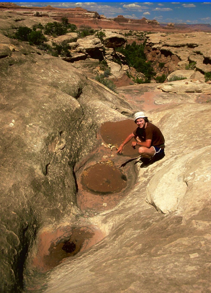
Tadpoles of oviparous Spadefoot toads (an Amphibian) in ephemeral pools in Canyon Lands National Park, Utah. The tadpoles must complete their metamorphosis before the pools dry up. Amphibians are mostly egg-layers. Most female amphibians lay a gelatinous mass of eggs in water, but a few species place the eggs in damp forest floors under vegetation or detritus or even carry them on their backs. Most frog’s and toad’s eggs develop and hatch in the water. There are a few exceptions. The terrestrial, Mexican caecilian and the aquatic cayenne caecilian give birth to fully metamorphosed live young. The embryos are nourished with secretions they scrape off the walls of their mothers’ oviducts. There are a few species of frogs, toads and salamanders that have a similar strategy as the caecilian.
they break out or hatch as tadpoles feeding on detritus and then metamorphose (gain legs and lungs and lose their tail and gills) in preparation for amphibious life. Around the U.S. toads are more terrestrial than frogs, but both pretty much lay eggs in water.
Fish are so diverse and there are so many species they show all three birthing patterns. Most are egg layers. The harsher and the more dangerous their environment then the more eggs they produce. Fish that guard their eggs produce smaller clutches. There are ovoviviparous and viviparous species. Despite their primitive nature, there are shark species that are ovoviviparous and even some viviparous species. The living fossil, the Coelacanth which was thought extinct 70 million years ago turned out to be a live bearer.
-
What Your Father Never Gave You But Mitochondrial Eve Did
No the answer is not the “Y-Chromosome.” True that a father does not pass a Y-chromosome to his daughters, but as it pertains to all his children (male and female) the answer is “Mitochondria.” Mitochondria are the sub-cellular organelles that process our energy. It is where energy from broken-down food molecules are converted to “ATP” the life-universal molecule for energy processes. The energy in the chemical bonds of the food substances which we ingest is converted into the energy of the bond of the third Phosphorus of Adenosine Tri-Phosphate (ATP) by the addition of a third Phosphate to Adenosine Di-Phosphate. It is a very complex process taught to all Biology Majors. An ATP molecule is like a “charged battery”. When ATP is converted to ADP (Adenosine Di-Phosphate) the energy from the third bond is used to do work (i.e., life processes). We need ATP for virtually everything we call life. We need it for muscle contraction, nerve impulse firing, thought, sight, everything we do. But this blog is not about physiology, it is about mitochondria. All higher plants and animals which have cells with a chromosome-bearing nucleus have mitochondria (the enlarged bean shaped organelle shown on left in diagram below) in the cell’s (the upper right in the diagram below) cytoplasm. The cytoplasm is the fluid filled area in cells between the nucleus and the outer cell membrane. The cytoplasm has a variety of “organelles” one of which is the mitochondria.

Mitochondria have their own circular, bacteria-like DNA And the cells have lots of mitochondria, 100’s or even 1000! Cells which consume more energy have more mitochondria. Bacteria and related primitive life forms do not have organelles so they do not have discrete mitochondria. In fact they do not have a discrete nucleus with chromosomes. Bacteria, cyanobacteria (blue-green algae) and the bacteria-like algae that live in hot thermal springs also have circular DNA, and internal membranes that function like our mitochondria for energy metabolism. Now here is the first interesting fact. There are between 2 and 10 or so circular DNA’s inside our mitochondria which are remarkably like bacterial DNA. Our mitochondria duplicate their DNA and divide into two mitochondria pretty much like bacteria replicate their DNA. Studies of the specifics of the “genome” of bacteria and mitochondria have led most biologists to accept the “Endosymbiotic Theory” of the origin of the cells of higher plants and animals. It is believed that perhaps 1 to 2 billion years ago a primitive cell life form engulfed another and rather than consume or digest it, the engulfed primitive cell was retained in a symbiotic relationship. And over 1.5 billion years the relationship of the engulfed cell (today’s mitochondria and chloroplasts) to the host cell has evolved.
The endosymbiotic theory of mitochondrial origin is nowadays well confirmed and it is believed to be related to the increase of oxygen level in the atmosphere. The size of the symbiont’s genome was reduced due to endosymbiotic gene transfer (EGT) or gene loss during evolution. Genes involved in the synthesis of nucleosides (any one of the four nitrogenous bases bonded to a 5-carbon sugar like ribose or deoxyribose) and amino acids, anaerobic glycolysis, and cellular regulation were conveyed to the host and are currently encoded by nuclear DNA (nDNA) in humans.
And thus the first mitochondria-like organelle appeared in a primitive nucleated organism. Similarly, plant’s chloroplasts (where photosynthesis occurs) have circular DNA. It is also believed that a primitive photosynthetic organism much like today’s blue-green algae (cyano-bacteria) was engulfed and became a symbiotic photosynthetic organelle for the evolutionary precursors of higher algae and plants.

The Endosymbiotic Theory For Origin Of Mitochondria Now back to what our fathers did not give us. A sperm does not contain any mitochondria which merge with the mitochondria of an ovum. A sperm contains 50–75 mitochondria in its midsection. The sperm’s mitochondria produce energy for the movement of the sperm. For comparison, in humans, the mature egg cell, or oocyte, contains from 100,000 to 600,000 mitochondria per cell, but each mitochondrion contains only one copy of mitochondrial DNA (mtDNA) initially.
A sperm has just enough mitochondria so it can swim so-to-speak, but it just passes an “N” or haploid set of chromosomes to the ovum. We get all our mitochondria from our mothers, who got theirs from their mothers, and so on and so on, infinitum. We have sequenced our mitochondrial DNA. It will be exactly like our mothers except for any mutations. And it will be like your grandmother on your mother’s side. And so on, and so on. The mitochondrial DNA measures only about 16,569 DNA base pairs (compared to 3.2 billion for your nuclear DNA in your chromosomes) and because it is circular and not a chromosome it does not re-combine (another future blog for Genetics Students). So mitochondrial DNA is quite useful for mapping human populations. Tiny mutations and changes in mitochondrial DNA in human populations traveled with the human populations as humans spread out over the earth from east-central Africa about 150,000 years ago. The companies that provide you with information about your genetic heritage use the mitochondrial differences along with nuclear chromosomal DNA markers to give you a genetic makeup.
Mitochondrial Eve – She is a theoretical woman who existed more than 150,000 years ago and all mitochondria in humans today can be traced back to her. Mutations in mitochondrial DNA (mtDNA) happen at a predictable rate in human populations. This is the so-called “clock.” Evolutionary geneticists look at the rate of mutations and changes in mtDNA across human populations and estimate that Mitochondria Eve existed 150,000 years ago. In order to be “Eve” she must have one or more female children who in turn had one or more female children and so on and so on until modern times. A woman who has no children or only male children could not pass on her mitochondria. If she or all of her female children and their female children died prior to having a female child, then she could not pass on her mitochondria. It is believed that human populations have experienced several bottlenecks where our numbers probably became quite low. In reality, a Mitochondrial Eve is not the first female of the human species, but merely the most recent female historically from which all humans can trace their mitochondrial ancestry. Mitochondrial Eve probably was a member of one of the small bottlenecked populations and likely located in east central Africa which is believed to be the cradle of humanity. Mitochondrial Eve dates back to around 100,000 to 250,000 years ago; the large range is indicative of the statistical variance of the data. Considering the history of human mitochondria, opposition to “three party babies (next blog) ” seems unfounded since the opposition is about mitochondrial DNA.

Mitochondrial Inheritance (Right) As human populations migrated out of Africa they took with them the mitochondria which would be shared by the entire human population on earth. Small subtle changes in the mitochondrial genome would be carried with the migrations of people and are present today in our mitochondria. The various ancestral DNA companies use these small differences was well as our nuclear DNA to trace our family’s origins.

The movements of humans across our planet. -
Variety Is The Spice Of Life…. Literally…

The Northern Elephant Seal (left) and it current range. “Variety’s the very spice of life…” was a quotation from the English poet William Cowper (1731–1800) in The Task (1785). For biologists whose specialty is “Conservation Biology” it means that maintaining genetic diversity in a species is in the best interests of the species’ long-term survival. Genetic diversity in turn means maintaining many different “alleles” or versions of genes (previous blog) in a species’ population and in the populations of that species throughout the species’ geographic range. The theory is that a species evolves or is adapted to subtle differences in its environment throughout its geographic range and that these adaptions are made possible by equally subtle changes in its genome (previous blog). That is, the genetic modifications fine tune the species to different conditions dictated by differences between the habitats throughout its geographic distribution.
Biodiversity vs Genetic Bottleneck.
Widescale habitat loss (e.g., deforestation of the Amazon basin) leading to fewer total number of different species is referred to as loss of biodiversity. Loss of a single species’ populations is termed “genetic bottlenecking” or a “genetic bottleneck” when the losses constitutes a large proportion of the species.
The two most common ways that a species experiences loss of genetic diversity due to humans are: 1) over-exploitation and the resultant reduction in the species abundance, and 2) habitat fragmentation which results in isolated populations which prevents genetic exchange between adjacent populations. Natural means of loss of genetic are founder populations and isolation by means of geologic processes.
Two Extreme Examples Of A Genetic Bottleneck By Over-Exploitation: The Northern Elephant Seal and The American Bison
The Northern Elephant Seal was hunted beginning in the 1700’s for their oil-rich blubber, which was used to make oil for lamps and lubrication. It was thought extinct in the late 1800’s but about 100 elephant seals remained on Guadalupe Island off the coast of Baja California in 1892. This small residual population is the source of all Northern Elephant Seals (see map below). All the allele diversity which was present in the historic populations up the North American coast were lost. Those alleles are gone forever. Today, the northern elephant seal population has rebounded to approximately the size it was before hunting. It’s estimated that there are about 150,000 individuals all derived from the 100 which survived on Guadalupe Island. The Northern Elephant Seal is an example of a highly bottlenecked species.
The American Bison – The American Bison. Bison once ranged from Florida to Maine and west to the Rocky Mountains of North America. Several sub-species existed including a slightly smaller woodland bison here in the Eastern U.S. The Bison was extirpated from the east and nearly extirpated from the Great Plains and western U.S. No exact population counts were made but most experts agree that there probably were 30 million bison before European settlement and westward expansion. By 1900 the bison was nearly extinct. Thirty million Bison to only 325 in 1884 to 500,000 today. There may be 500,000 Bison but genetically speaking, the effective size is much smaller.

The American Bison Then and Now There are formulas which Conservation Biologists use to calculate the “effective population size” based upon the “bottleneck” (e.g., the mid to late 1800’s for the American Bison. The roughly 5,000 bison roaming the Yellowstone National Park today are descendants of just two dozen individuals that found a haven in Yellowstone’s rugged interior.
In 2015, a purebred herd of 350 individuals was identified on public lands in the Henry Mountains of southern Utah via genetic testing of mitochondrial and nuclear DNA. Efforts are being made to diversify the genomes of the Bison’s fragmented populations. The American Bison is genetically bottlenecked. We will never get the Eastern Woodland Bison of the Southeast U.S. back. The European Bison (the Wisent) is also bottlenecked genetically. Historically, the European bison’s range encompassed almost all of Europe, including southern England, and Russia.
African Mega Fauna – A genetic bottleneck also occurs when a species’ populations become fragmented. This occurs because of the physical distances between populations. Alleles can’t be shared between fragmented populations because individuals at the edges of populations can no longer breed with adjacent populations. The African Lion is a good example of a highly fragmented species. It once roamed over most of sub-Saharan African but now is highly fragmented. Of course other large mammals (e.g., African Elephant) in Africa have experienced the same population fragmentation.

Fragmentation of African Lion Populations; CONSERVATION STRATEGY FOR THE LION IN WEST AND CENTRAL AFRICA ; Prepared by the IUCN SSC Cat Specialist Group 2006 Founder Populations – When a small subset of a species migrates to an area which it previously did not occur in and establishes itself there the migrants take a small subset of the allele diversity present in the source population. This can create a genetic bottleneck and can drive evolutionary change. It is believed that birds that populated the remote Galapagos Islands were probably “founders” from mainland South America and that they subsequently took unique evolutionary paths. Population bottlenecks are believed to lead to rapid changes in gene/allele frequencies through genetic drift, to facilitate rapid emergence of new phenotypes, and to enhance reproductive isolation. For such effects to occur, founding populations must be very small.
The Devil’s Hole Pupfish – In the desert southwest near Death Valley (California/Nevada) a unique example of fish evolution by means of isolation exists. During a wetter period in the geologic history of North America related to glaciation large inland seas existed in what is now Death Valley. One sea was “Lake Manly” and fossils show a single species of small fish in the genus Cyprinodon. Over 10’s of thousands of years the area became arid and the inland seas turned into dry “flats”, small streams and isolated pools fed by groundwater. The most extreme example is Devil’s Hole where there is now one unique species, the Devil’s Hole Pupfish (Cyprinodon diabolis) . The pool it lives in (Devils Hole) is about 72 ft long by 11.5 ft wide. The fish feed on a small shelf with algae growing on it because the shelfs exposure to sunlight for part of each day. The entire population of this species is about 200 and fluctuates. For decades depletion of groundwater from the aquifer has threatened this species with extinction.

Devils Hole, Ash Meadows, NV was once covered by an inland sea. Addendum For Genetics Students: Computing Effective Population Size, Ne.
Calculating Effective Population Size Ne:
Effective Population Size = Number of Generations / Sum of ( I /Ni )
where Ni = Population Size for ith generation.
Number of Generations in Data / SUM (1/Ni)
where Ni is population size in ith generation
Using this formula for the following data. Suppose a population of animals went from 1000 to just 10 and then recovered to 2000 in span of five generations (e.g., 1000, 10, 100,1000, 2000).
Ne = 5 / [ 1/1000 + 1/10 + 1/100 + 1/1000 + 1/2000 ]
Ne = 44
Work Problem:
The Norway Beaver was extirpated from most of its range just as the American Beaver was.
The remnant population of beaver in Norway, for example, grew from a precariously low 100 or so individuals in 1880 to 7,000 by the 1930s; not only providing ample numbers to spread across the country, but also for reintroductions into neighboring Sweden and nearby Finland.
Presently an estimated 70,000.
1880, 100 beaver
1930, 7000 beaver
1960, 30000 beaver
2000, 70000 beaverEffective Population Size =
ANSWER: N=4/(1/100 + 1/7000 + 1/30000 + 1/70000) = 392
-
De-Extinction – Bringing Back The Wooly Mammoth

The Wooly Mammoth painted by Mauricio Antón Ortuzar, a paleoartist and illustrator specialized in the scientific reconstruction of extinct life. The general public was first introduced to this concept of de-extinction in the blockbuster film Jurassic Park (1993). Present efforts at de-extinction are focused on more modern animals rather than dinosaurs. The reason being the availability of complete DNA. The biology behind de-extinction actually has several components: cloning technology, gene sequencing, and gene editing (called CRISPR; say “crisper” like how you might order fries with your burger). De-extinction efforts presently involve the Wooly Mammoth and the Tasmanian Tiger (which was actually a Marsupial predator about the size of an un-related wolf).
Wooly mammoths became extinct possibly as recent as 5000 years ago. Melting ice has exposed many frozen specimens and provided enough DNA to sequence their entire genome. Wooly mammoth’s nearest living relative is the Indian Elephant according to its genome (genome: previous blog). Efforts to re-create the Wooly Mammoth are two-fold and the two approaches differ. First is conventional “modern cloning”. South Korean scientists have successfully cloned many dogs. Use Google and search on “Suppy” a cloned Afghan dog. Suppy’s clones have been cloned. The rich and famous in Hollywood have had their dogs cloned. This approach for the Wooly Mammoth would take a Mammoth cell with intact DNA from the Mammoth and then extract the nucleus with its full set (2n) of chromosomes. An ovum from an Indian Elephant would be de-nucleated (but the remainder of sub-cellular organelles left intact in the ovum). The Wooly Mammoth’s nucleus is inserted into the Elephant ovum and proprietary technology is used to cause the ovum to start dividing. It is implanted into the uterus of an Elephant which will act as a surrogate mother. With elephants, gestation and maturation to adult body forms is a decades long process. The idea is to first produce a small herd and then allow them to grow into more herds of mammoths.

The second approach for the Wooly Mammoth is to use the gene editing technology of CRISPR to edit into the Indian Elephant’s genome those portions of the Wooly Mammoth’s genome that are different. The Indian Elephant as well as African Elephant’s genome have been sequenced. The goal is to produce a “Wooly Elephant.” Through selective breeding and more gene editing it is believed that something pretty close to a Wooly Mammoth would be produced. CRISPR technology allows genetic engineers to cut out and replace very specific portions of a creature’s genome and either render it “non-expressed” or edit it “improved.” As long as the cut/repair is accurate all is well. If it is off-target then bad things happen such as rendering an adjacent gene non-functional. CRISPR uses bacterial enzymes to make the cut and splices. The enzymes which make the cuts utilize a manufactured guide molecule of RNA which is very specific and will only position the cutting enzyme at the intended point of the genome. The key to success being SPECIFICITY, such that changes to the genome (previous blog) are accurate. There are several human genetic diseases that are simply one single base change in the human genome; one out of 3.2 billion! If you could apply CRISPR to fix the genetic error in a sperm or ovum, then a parent would not pass the genetic disease to their children.
How different are the genomes of Wooly Mammoth vs Indian Elephant? Asian elephants and woolly mammoths share a 99.6 percent similar DNA. For comparison, humans and chimps share a 98.8 percent of their DNA. Despite the close percentages there are lots of differences. Humans and a banana share 44% of our genomes! This is because so much of an organism’s genome is for basic shared cellular processes related to energy metabolism.
Efforts for de-extinction of the Tasmanian Tiger (Thylacine) also known as the Tasmanian wolf, will be a bit more complicated. (Note: Tasmanian Tiger are not related to tigers and are not related to wolves. They are also not related to Australian Dingos which are derived from domesticated dogs which early man brought to Australia from neighboring islands during human population expansion. There is speculation that they may still survive in some remote regions. The last known Tasmanian Tiger died in a zoo in 1936. Tasmanian Tigers are marsupials so a marsupial will have to be selected to serve as surrogate mother. Embryonic marsupials are very poorly developed when they crawl from the uterus into the mother’s pouch. Finding a suitable surrogate from among exiting marsupials will present a challenge. An alternative approach which scientists might use is to replace the surrogate/pouch phase with “bottle” feeding milk to the tiny embryos.
CRISPR ADDENDUM FOR GENETICS STUDENTS
A Quick Overview Of CRISPR
CRISPR – stands for “clustered regularly interspaced short palindromic repeats” These sequences are present in bacterial genomes and represent fragments of former viral infections of the bacteria. They are used by the bacteria to destroy viruses that infect the bacteria. CAS-9 (or “CRISPR-associated protein 9”) is a bacterial enzyme that uses the sequences to target invading viruses and destroy them by cutting the viral genome. There are other “CAS” enzymes. So what if you could “guide” CAS-9 to a specific location in an organism’s genome and make a cut. The cut would be guided not by fragments of former viral infections as is the case in bacteria, but it would be guided by man-made guide RNA designed to align with a target area of the organism’s gene and make a cut or edit. As you will see we will need: 1) the CAS enzyme, 2) a man-made carrier or guide piece of RNA which can carry the CAS enzyme and has a man-made sequence that will base-pair with the gene at the intended cut site, and 3) a “PAM” (e.g., GCC) in the proper place (see PAM BELOW). Suppose that you want to change the genome at the location indicated by the larger font:

The target for the cut The bold italic portion located to the left of the intended cut provides a VERY specific 23-base pair target. Since the human genome is known and there are websites where one can search the entire human genome for a sequence one can verify that there are no un-intended portions of the genome that have the same “target.” And it has the so-called PAM (Protospacer Adjacent Motif (which is 2-6 base pairs in size) GCC at the right side of target which is specific for the cutting enzyme (CAS-x). What is needed now is a guiding molecule that will take the cutting bacterial enzyme “CAS-x” to this VERY specific point in the genome. Without the “guide” the cutting enzyme will never make a cut. Since we know the base or genome sequence at the planned cut-location we synthesize a guide piece of RNA which will match up with the DNA at the planned cut location.

This is the guide RNA which will align with the target portion of the DNA. When the two strands of DNA separate the guide RNA will pair with the DNA and position CAS-9.

The guide RNA will position the CAS enzyme at the PAM and the enzyme will cut at the “G” -
Familia DNA, CSI And A Cigar Left On The Street

This is the story of three living grandsons or “cousins” but only two were known to each other and to the family. One of these two committed a murder but it was his half-brother unknown to the family who was arrested, convicted and was serving time for murder.
A man (Grandfather Y) and a woman (Grandmother X) had three sons in the 1940’s. These three sons were adults around 1970 but are no longer alive. The blue icons in the family tree are three women who were outside the family and had the grandsons of Grandfather Y and Grandmother X. Woman Gamma was unknown to all but Son 1. Son 1 had a son (Grandson B) with Woman Alpha. Grandson B was known to the family. Son 1’s brother (Son 3) had two sons but only one (Grandson C) is alive (Grandson D was killed in an auto accident). Grandson C was only aware that he had a cousin but had not seen him in quite some time and believed his cousin Grandson B lived New York City (in fact Grandson B left for NYC after committing the crime). Woman Beta who was still alive told also thought her nephew lived in NYC.
Son 1 had another son with another woman (Woman Gamma). His wife (Woman Alpha) was never aware of this other son. None of Son 1’s brothers, sister in-law or nephews were ever aware of his son, Grandson A.
Thus, Grandson A and Grandson B are half-brothers but never knew about one another (their mothers also were unaware of each other’s existence). Grandson B committed a murder around 1990 in a high-profile case. He fled the area to New York City, was unknown to local law enforcement where the crime occurred and was thus never considered as a suspect. Grandson A had a few non-violent crimes to his record and was arrested and confessed to a murder he did not commit. One witness to the crime identified him in a lineup (half-brothers would be expected to show some resemblance, but he was unaware of his half-brother). At the time DNA analysis did not exist as it does today. Sets of enzymes in his blood, blood type and the witness testimony were enough evidence to get him to sign a plea agreement. He was convicted and sentenced to life without parole as part of the plea agreement. Flash forward 20 plus years when we have modern DNA analysis and ancestral DNA analysis. There are “projects” where lawyers strive to use modern science to correct bad arrests and convictions using modern forensic DNA analysis and archived DNA samples remaining from former crime scenes. Grandson A’s DNA proves to be only about a 23% match with the crime scene tissues suggesting that perhaps an aunt, uncle or half sibling committed the murder. But there are no known living blood-line aunts or uncles. The crime scene samples were compared to data in the databases of ancestral DNA data.
An 11% match is found in what initially seemed to be an un-related family. Grandson C had submitted DNA for a family DNA analysis. The only living relatives of Grandson C was his elderly mother (Woman Beta, who married into the family tree) and a cousin he hardly knew. Grandson C was unaware he had another cousin, Grandson A. He told investigators he thought his cousin Grandson B now lives in NYC. NYC Law Enforcement were familiar with Grandson B because of a number of minor criminal arrests. Investigators locate this cousin (Grandson B) in NYC and collect a cigar he tossed on the street. There is no expectation of privacy for data collected from littering a cigar. DNA on the cigar is a 100% match to the crime scene DNA from decades before. It took a while, but the courts overturned the original conviction and Grandson A is released after serving 20 years for a murder committed by his unknown half-brother. Many similar cases have used even lesser shared DNA levels (2nd and 3rd cousins) to narrow down lists of probable suspects and have led to successful cold case closures.
-
What is your genome? You have heard the term on the news.
Humans have 23 pairs (i.e., 2n) of chromosomes in each of their somatic (non-reproductive) cells which have nuclei. (Note: Sperm and ova have 23 unpaired chromosomes because the number has been halved (i.e., from “2n” to “n” on order to produce the gamete; the process of meiosis). A picture of the 23 pairs of chromosomes is a Karyotype

Human Diploid Chromosomes (male set; M=Maternal, P = Paternal) Each pair is said to be a “homologous pair” because they contain the same genes at the precise same locations (i.e., loci) along the chromosome. But they might and probably do contain different versions of the gene. The technical name for different versions of the gene are “alleles.” Of course the reason you have two of each homologous chromosome is one came from your father’s sperm and one from your mother’s ovum (again, a sentence that made my college students squirm).
The shapes of the chromosomes depicted in the photo of the karyotype is how they appear when cells are dividing. Normally when the cells are not dividing from one into two cells (the process of mitosis) they are much (many orders of magnitude) thinner and longer. The DNA which is continuous and linear along the length of each chromosome is highly coiled and wrapped in proteins called histones. The DNA is a double helix meaning it is like a twisted and tilted ladder. I will use a ladder to describe DNA’s structure. The left and right side rails of the ladder is comprised of building blocks. Each unit of the building block is a phosphate and 5-carbon sugar (deoxyribose) which can be likened to the ladder’s side rails (vertical). Each sugar-phosphate building block also has one of four “bases” attached more or less perpendicular to the side rail which serves as half of each step. The bases are: Adenine, Thymine, Cytosine or Guanine (A,T,C or G). Every base (one half of each step) is bonded to a base on the other side of the “step”. So a “step” consists of two bases. Adenine always bonds to a Thymine (A-T or T-A) and Cytosine always binds to Guanine (C-G or G-C); see the illustration below. In the discovery of DNA’s structure (last post) Crick and Watson were familiar with the research of anscientist named Chargaff who lectured at Cambridge in 1952 with Watson and Crick in attendance. He showed that human DNA had equal Adenine and Thymine quantities and equal Cytosine and Guanine amounts. Watson and Crick used this fact to build a model where A bonded to T and C bonded to G in the model.

If you could un-coil and un-twist a chromosome and then divide it into its left and right sides you would be left with two extraordinarily long series of the bases since the stair’s left and right sides of the steps were separated. The letters might be AATGGCTATTCCCGATAGCCGA….and if written all the way out it would be perhaps 150 millions characters long for an typical chromosome.
By the way, “Gattaca” is a 1997 American dystopian science fiction film starring Ethan Hawke, Uma Thurman and Jude Law. The film’s name is a reference to genomes.
A gene consists of a sequence of 1000’s of the bases so any single chromosome contains hundreds or even more than 1000 genes plus or minus. The 23 chromosomes differ in their gene density. Chromosome number 1 is not only the longest but contains almost 3000 genes, more than any other. Guys, the Y chromosomes has the least number of genes, about 100. About 30,000 genes have been identified in humans and there are 23 chromosomes so you can do the math. Genes actually have “start” sequences and “end” sequences which is a necessity in order for genes to be expressed at times and not expressed at other times based upon the physiological state of the tissue and developmental state of the creature. For example the need for the enzymes to digest a meal are needed based upon the timing of food intake. The digestive enzymes are proteins whose composition is coded by the four bases in the sequence of your genome where the gene for that particular enzyme is located. Physiological signal molecules act to enhance the expression of the gene.
Your genome is the combined list of all the bases as they appear in sequence across all 23 chromosomes. It consists of about 3.2 billion characters from just four letters A, T, G and C. Of course there is meaning to all the letters because a gene typically consists of 1000’s of the letters, and in sets of three letters they define the order that amino acids are assembled into proteins in tiny sub-cellular organs called “organelles” in the cell and outside of the cell’s nucleus. The interpretation of a gene into a protein is called “translation.” The letters of the DNA are “transcribed” into complimentary letters in the messenger RNA (mRNA) which travels out of the cell’s nucleus and is “translated” into a protein by joining amino acids in the sequence defined by the letters (bases A,T,C and G) in the mRNA, read three letters at a time.
The technology to determine those sequences of millions and millions of bases (A,T,C and G) is amazing. It starts with amplifying a small amount of the genome into millions of copies in a process called “PCR” which stands for Polymerase Chain Reaction. The “chain reaction” part eludes to the amplification of the amount of DNA, not the use of radioactive materials! Then the chromosomes are literally blasted into millions fragments, sequenced and then re-assembled mathematically. (For Genetics Students: both strands are read in the 5’ to 3’ direction). Since genes have start and stop sequences defined by three bases the software of the super computers which reassembles all the data recognizes which sides of the ladder so-to-speak go with one-another. The “PCR” process owes it ability to an enzyme discovered in heat-loving bacteria in very hot thermal springs. The bacteria is names Thermus aquaticus and was first isolated from Mushroom Spring in the Lower Geyser Basin of Yellowstone National Park. The heat-stable enzyme is named TAQ Polymerase where “TAQ” is a reference to its Latin name (the T from Thermus and the AQ from aquaticus). Every DNA test in the world starts with PCR using the enzyme followed by DNA sequencing which in itself is an amazing technological and mathematical achievement.
Finally, DNA is being used for data storage. DNA is synthesized and the order of the bases is used to produce information just like the 1’s and 0’s in conventional memory chips. But the data density is spectacular. It is estimated that all published materials could be encoded into DNA and fit into the trunk of a medium automobile. The DNA is good for dense long-term data storage but can’t be read as fast as solid state chips.
-
Women’s History Month – Rosalind Franklin

Rosalind Elsie Franklin (25 July 1920 – 16 April 1958) March is Women’s History Month. Rosalind Franklin was a key figure in the discovery of DNA’s structure. She was an X-Ray Crystallographer who was working at King’s College in the UK at the same time as Watson and Crick who were at Cambridge. This all took place during the transition of King George VI of England and Queen Elizabeth. At the time, biologists knew there were such things as nucleic acids in cell nuclei and that genes were the “stuff of inheritance” but scientists were clueless as to how DNA was structured and “what was a gene”. Remember that patterns of predictable inheritance of genes had been worked out by Gregor Mendel decades before in the late 1800’s but in the early 1950’s nobody knew what a gene was. Watson (British) and Crick (a visiting USA researcher) were attempting to determine the structure of DNA. They were virtually doing it in their spare time as they had other research roles at The Cavendish Laboratory at Cambridge. They were more-or-less stuck, their physical models of DNA just did not fit (i.e., the physical constraints of the molecules Adenine, Thymine, Cytosine and Guanine along with deoxyribose (5-carbon sugar) and Phosphorus did not arrange properly). Watson traveled to King’s College because he and Crick had heard about Franklin’s successes in using X-ray crystallography to determine the shape of DNA. Rosalind Franklin’s supervisor at King’s College was Maurice Wilkins. Franklin was opposed to prematurely building theoretical models, until sufficient data were obtained to properly guide the model building. Wilkins gave Watson a more-or-less unauthorized peak at Franklin’s’ famous “Photograph 51” (below).

While returning on the train to Cambridge Watson scribbled down a diagram based upon his brief viewing of Photograph 51. When he showed his drawing to Crick it was a watershed moment because Watson immediately recognized it as a double helix. Crick had taught himself the mathematical theory of X-ray crystallography. Also, Crick’s access to a progress report by Franklin late in 1952 made Crick confident that DNA was a double helix with antiparallel chains (for students of Genetics, see the technical addendum below).
Watson and Crick finished building their model on 7 March 1953. To be fair Watson might not have completed the model if he had not got a vital tip from the son of U.S. scientist Linus Pauling. Pauling senior in the U.S. was also attempting to define the structure for DNA. Pauling’s son was visiting in Cambridge and told Watson that he was using the wrong forms of the four bases and he should talk to Jerry Donohue, an American crystallographer who was also working at Cambridge at the time. The bases occur in “enol” and “keto” forms which affects their size and symmetry. Watson and Crick had been building their model with “enol” shapes that did not fit. When Watson started cutting out cardboard molecules using “keto” dimensions it worked! A beautiful, symmetrical, twisted and tilted double helix emerged!

Watson and Crick together developed a model for a helical structure of DNA, which they published on 25 April 1953 in the journal “Nature.” Franklin viewed their model in early April. She was gracious and remarked on its beauty and simplicity. She also published an article of her X-ray work in the same issue of Nature (this was an arrangement to recognize properly her contributions).
In 1962 the Nobel Prize was subsequently awarded to Crick, Watson, and Wilkins (they had been nominated in 1960 and 1961). Nobel rules now prohibit posthumous nominations (though this statute was not formally in effect until 1974) or splitting of Prizes more than three ways. Later, Franklin commenced deciphering the structure of the polio virus while it was in a crystalline state but was forced to end her work due to her rapidly failing health. Rosalind Franklin died in 1958 from cancer. After her death, her research group headed by Klug completed the polio virus work and published the results in 1959. Klug was the sole winner of the Nobel Prize in Chemistry 1982 for his work he started while working for Franklin. This work was exactly what Franklin had started and which she introduced to Klug, and it is highly likely that, if she were alive, she would have shared Klug’s Nobel Prize. Rosalind Franklin’s photo called “Photograph 51” probably was the single most important discovery which accelerated the discovery of DNA’s molecular structure. What followed was Crick’s “Central Dogma” where the bases of DNA dictate the bases of RNA which in turn define the sequence of amino acids in proteins.
Actress Nicole Kidman portrayed Rosalind Franklin on stage in “Photograph 51” Kidman won at the 2015 London Evening Standard theatre awards for her portrayal of the overlooked DNA scientist Rosalind Franklin in “Photograph 51.”
Life Story (also known as The Race for the Double Helix in the United States) is a 1987 television historical drama which depicts the progress toward, and the competition for, the discovery of the structure of DNA starring a young Jeff Goldblum as Jim Watson (the US half of Watson and Crick).
Addendum For Genetics Students
Antiparallel means that one side of the DNA is oriented 5’ to 3’ and the other 3’ to 5’ where 3’ and 5’ are Carbon molecule positions on the 5-carbon sugar molecule deoxyribose in DNA. In other words, the two sides are pointed in opposite directions.

The X-Ray Crystallography (photograph 51) performed by Dr. Franklin showed that DNA was 20 Angstroms wide and that bases were 3.4 Angstroms apart. Every 10 bases or every 34 Angstroms DNA makes one complete turn. The complete turn includes what are termed “minor grooves” and “major grooves.” In deoxyribonucleic acids (DNA), the nucleotide bases guanine and thymine are in keto form, and adenine and cytosine are in amino form (20 Angstrom width for the pairs). Dr. Franklin had also reported that the dark shadows outside the X-pattern in Photograph 51 were likely due to Phosphorus being on the outside of the DNA molecule (i.e., the outside of the double helix with the bases being in the inside).
Watson and Crick were familiar Chargaff’s observation that the molar amounts of A and T are always equal, as are G and C in DNA. The trick was building a model for the molecule. Watson and Crick were building models using the wrong tautomers (e.g., enol and imino forms) of the bases (since those were the structures in textbooks) until the organic chemist Jerry Donohue (a laboratory partner) told them to use the keto form of thymine and guanine and the amino forms of adenine and cytosine. In the enol/imino forms these two bases could not fit a 20 A DNA molecule. But in the keto/amino forms they fit the 20 Angstrom model predicted by Photograph 51.


Science and Nature by JW Foltz
Science, Nature and the Environment
“…when the last individual of a race of living things breathes no more,
another heaven and another earth must pass before such a one can be again” C. William Beebe, 1906.
“
